Rectangular pseudopolyconic projection for geographical maps

Regions lying far away from the Equator at medium and higher latitudes, are represented on geographical maps mostly in conical or pseudoconical projections showing parallels as circle arcs. The graticule in conical projections is orthogonal, that is meridians intersect parallels perpendicularly, but this does not hold true of most pseudoconical projections used practically in geo-cartography (e.g. Bonne projection, ordinary polyconic projection).

There are some pseudoconical projections with orthogonal graticule used for topographical maps (e.g. "War Office" projection spread in Great Britain in the 19^th c., the modified polyconic applied in Canada [3]). The advantage is that they are not conformal, however their angular distortion is not significant because of the orthogonality, in addition errors rising from linear and area distortion cannot increase so much as on maps with conformal projection.

There is reason to apply the orthogonal polyconic projection for geographical maps, if the mean of the errors may be diminished. To clear up this, first of all it is to be decided, which distortions are regarded as disadvantageous from the point of view of the topic of the map. If there isn't such distortion to be avoided, then all distortions (namely linear, angular and area distortions) must be taken into account in some summarized form; the so called overall mean error criteria serve for this purpose. The value of these indexes are to be reduced to the possible highest pitch in case, if more topics with several distortion claim are to be represented on a map series of the same territory.

The conical and pseudoconical projections show the parallels as circle arcs. The mapping equations are:

 ,

where  r=r(b)  is the radius of the parallel  b  on the map;  c=c(b)  is the distance of the centre of the paralel  b  from the axis  x; g=g(b,l)  is the angle of the radius-vector pointing to the image of the point  (b,l) enclosing with the central meridian, which is a strictly monotonically increasing odd function of  l. (b=90°-j ,  where  j  is the latitude;  l  is the longitude.)

It is known ([1]) that for the conical and the regular pseudoconical projections cºconst,

that is the images of the parallels are concentric circle arcs, moreover for the conical projection, where costant  n  is the meridian inclination (0< n <1). For the polyconic projection, the radius of the parallels on the map is: r=tgb.  It is a strong obligation, therefore – as it will be demonstrated later – from the point of view of distortions the polyconic projections are often unfavourable. The pseudopolyconic projections differ from the polyconic in the radius of the parallels:  r=r(b)  can be any arbitrary strictly monotonically increasing function.

Denoted by  q  the angle of the meridians and parallels, at the orthogonal projections  q=90°,  that is  ctgq=0.  On the other hand from the theory of the projectional distortions it is well-known ([1], [5], [6]) that the value  ctgq  for the pseudoconical projections can be calculated from the formula

 .

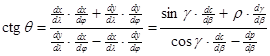Thereby, the equality

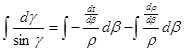
is valid at the orthogonal pseudoconical projections. It is a separable differential equation; its solution is

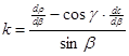
Let us rewrite the function  c(b)  in form  c(b)=t(b)+r (b). Then function  t(b)  giving the distance of the intersection of the parallel  b  with the central meridian from the axis x on the map (see figure 1), determines the scale k along the central meridian (l=0):

As it can often be seen at the pseudoconical projections, for practical purposes the function t(b) should be chosen as linear:  t(b)=t₁×arcb .  (Further on, the radian value of the angle  x   given in degrees will be denoted by  arcx .)  So the central meridian is equidistant, and if  t₁=1, then it is true scale. In the case of claim of greater accuracy the function  t(b)  can be approximated by a quadratic polynomial  t₁×b+ t₂×b ².

Continuing the solution of the above equation:

that is

 .

The radial function  r=r(b)  can be chosen linear or nonlinear. On the other hand, depending on whether the value of the constant in the radial function equals zero or not, the projection can represent the pole as a point or a line. Approximating  r=r(b)  by a quadratic polynomial according to the above the following cases must be taken into account:

a) r=r₁×arcb , linear radial function with pole as point (central meridian is equidistant)

b) r=r₀+r₁×arcb , linear radial function with pole line (central meridian is equidistant)

c) r=r₁×arcb+r₂×arc²b , quadratic radial function with pole as point

d) r=r₀+r₁×arcb+r₂×arc²b, quadratic radial function with pole line

where  r₀  is the radius of the pole line.

Then the function    is a rational fractional function, so it has primitive function.

Using the notation   , 

  results, putting the integration constant as  ln f(l) .

It follows from this 

and finally   .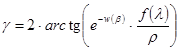

So depending on the form of the radial function  r=r(b),  g  can assume the following forms:

If  r=r₁×arcb  is  ;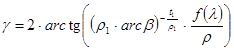

if  r=r₀+r₁×arcb  is  ;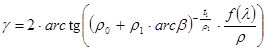

if  r=r₁×arcb+r₂×arc²b  is  ;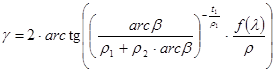

and if  r=r₀+r₁×arcb+r₂×arc²b  is 

 .

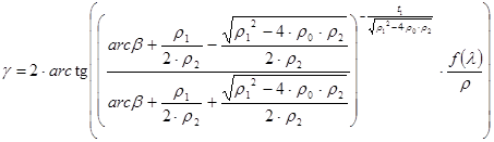The function  f(l)  is odd of  l ,  therefore it can be approximated by  f₁×arcl+ f₂×arc³l+ f₃×arc⁵l . The number of terms - mostly two or three - to be taken into account for the projection of a given map depends on the east-west extension of the territory to be represented.

With the knowledge of radial function  r=r(b),  distance  c=c(b)  and  angle  g=g(b,l) the overall error in an arbitrary point of the map can be appointed. To this the extremal scales a and b are needed. Because of the orthogonality their values correspond to the scales along the graticule h and k . Therefore the index of the local overall error of Airy-Kavrayskiy e²_AK   ([2]) can be calculated immediately from the scales along the graticule:

 ,  

and     

The formula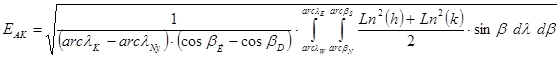 

gives the value of the Airy-Kavrayskiy's criterion of the mean overall error of E_AK  on a geographical quadrangle bordered by the parallels  b_N   and  b_S   as well as meridians  l_W  and  l_E.

Spacing the examined geographical quadrangle by a 1°x1° grid, the values  e²_AK×sinb  are calculated for the grid points. Summarizing them by the binary Simpson formula, dividing it by the area of the geographical quadrangle and finally extracting the root of it, this results in the suitably exact approximation of the criterion value  E_AK .

Further on two geometrical figures of different shape on the earth surface will be examined:

A) The territory of Canada more extended east-west, roughly covered by a geographic quadrangle between the parallels 45° and 75° N, as well as the meridians 60° and 140° W.

B) The more narrow, but longer north-south territory of the European Union, roughly covered by a geographic quadrangle between the parallels 35° and 70° N, as well as the meridians 10° W and 30° E.

For comparison these two territories were represented at first on equidistant conic projection of de l'Isle, then secondly on orthogonal polyconic projection, and at last on orthogonal pseudopolyconic projection explained before. (See the constituent functions of the two former projections and the optimal parameters in the appendix.) At the latter projection the radial function  r=r(b)  was taken into account in three versions  (r=r₁×arcb ,  r=r₀+r₁×arcb   and  r=r₁×arcb+r₂×arc²b); the calculations certified that the radial function of three parameters (r=r₀+r₁×arcb+r₂×arc²b) does not give better result, that is the mean overall error is not significantly lower. The function  f(l)  was applied as linear polynomial (f₁×arcl), then polynomials of third  (f₁×arcl + f₂×arc³l)  and fifth   (f₁×arcl + f₂×arc³l + f₃×arc⁵l)  degree. The values of   E_AK  attached to the two geographical quadrangle, calculated by downhill simplex method ([4]) are summarized in Table 1.

Table 1

Extent of geographic quadrangle:	A)  Canada 15°N £b £45°N 140°W £l £60°W
	f(l)=f1×arcl	f(l)=f1×arcl+ f2×arc^3l	f(l)=f1×arcl+ f2×arc^3l + f3×arc^5l
De l’Isle projection                r=r0+arcb	EAK=0.00737	-	-
Orthogonal polyconic proj.   r=tgb	-	EAK=0.01818	-
Orth. Pseudopolyconic proj.  r=r1×arcb	EAK=0.02012	EAK=0.00643	EAK=0.00642
Orth. Pseudopolyconic proj.  r=r0+r1×arcb	EAK=0.02011	EAK=0.00637	EAK=0.00636
Orth. Pseudopolyconic proj.  r=r1×arcb+r2×arc^2b	EAK=0.02010	EAK=0.00635	EAK=0.00628
Extent of geographic quadrangle:	B)  European Union 20°N£ b £55°N 10°W£ l £30°E
	f(l)=f1×arcl	f(l)=f1×arcl+ f2×arc^3l	f(l)=f1×arcl+ f2×arc^3l + f3×arc^5l
De l’Isle projection                r=r0+arcb	EAK=0.01003	-	-
Orthogonal polyconic proj.   r=tgb	-	EAK=0.00625	-
Orth. Pseudopolyconic proj.  r=r1×arcb	EAK=0.00817	EAK=0.00714	EAK=0.00714
Orth. Pseudopolyconic proj.  r=r0+r1×arcb	EAK=0.00596	EAK=0.00449	EAK=0.00449
Orth. Pseudopolyconic proj.  r=r1×arcb+r2×arc^2b	EAK=0.00588	EAK=0.00442	EAK=0.00442

Table 1 shows that on the territories of given size and shape the mean overall error of the correctly selected orthogonal pseudopolyconic projection is lower than that of the best equidistant conic projection of de l’Isle, and that of the best orthogonal polyconic projection. This difference is evident mainly at the more narrow territory B), where the mean overall error of the polyconic projection is merely 62.5% of the error of the conic projection, and the error belonging to the pseudopolyconic projection is less than half of it.

On the wider territory A) the error of the pseudopolyconic projection can be reduced to the 85% of the error of the conical projection. Conversely, a disadvantageous characteristic at the polyconic projections clearly appears here, too: the distortion features go wrong apace with broadening of the of the represented region. This shows itself up at the orthogonal pseudopolyconic so that with extending of the territory to east-west, it converges to a conical projection.

Comparing the error of the different orthogonal pseudopolyconic projections it is remarkable that the error of the versions with two parameters (accordingly the version with pole line, equidistant along the central meridian, and the version with pole as point and with uniformly changing scale along the central meridian) is practically equal for both territories.

On the other hand the value of the error is influenced by the terms of the polynomial  f(l). At the wider territory the linear polynom is not usable because of the very high error value. Applying a function  f(l)  of the third degree (with two terms), the mean overall error diminishes significantly for both territories. Accommodating a function  f(l)  of fifth degree, at the wider region the error can be further reduced slightly.

Doing calculations getting the best pseudopoliconic projection for the two regions, sporadically negative pole line radius coefficient  r₀  arose. It means that a parallel near the pole is mapped to a singular point, and the area from this parallel to the pole is not representable. In this case it is advisable to abandon the environs of the pole.

Summarizing the conclusions drawn from the Table: the orthogonal pseudopolyconic

projection can be offered to representing large territories (big countries, parts of

continents, possibly whole continents) lying far away from the equator on geographical

maps. Mostly the radial function with two parameters can be suggested. The version where the

pole is a point is favourable when mapping a region with rather north-south extension,

respectively if the pole itself is represented. The version with pole line is advantageous if the

mapped region is far away from the pole, too, or it extends first of all east-west.

Tables 2 and 3 represent Canada and the European Union on orthogonal pseudopoliconic projection with pole line and respectively with pole as point.

Appendix

The radial function of the equdistant conical projection of de l'Isle: 

r=r₀+arcb ,  where  ; 

the meridian inclination:  (b₁ and b₂ are the true scale parallels).

Representing the geographic quadrangle A)  (namely b_S =45°; b_N =15°;   l_W =140°W;

l_E =60°W, covering Canada)  the minimal mean overall error E_AK =0.00737  turns up when choosing  b₁ =20.7° and b₂ =38.0°, that is  j₁ =69.3° and j₂ =52.0°  (it means r₀=0.04546,  n=0.8687).

Representing the geographic quadrangle B)  (namely b_S =55°; b_N =20°;   l_W =10°W;  l_E =30°E, covering the Europen Union) the minimal mean overall error  E_AK =0.01003  turns up when choosing b₁ =26.7° and b₂ =46.9°, that is  j₁ =63.3° and j₂ =43.0° (it means  r₀=0.9872,  n=0.7958).

The radial function of the orthogonal polyconic projection: r=tgb ;

the distance  c  of the centre of the parallel  b  from the axis  x: c=d×(p/2 - arcb)+r ;

the angle  g  of the radius-vector pointing to the image of the point  (b,l)  enclosing with the central meridian:

g=2×arctg[ctgb×sin^db×(f₁×arcl+f₂×arc³l)].

Representing the geographic quadrangle A), the minimal mean overall error  E_AK =0.01818  turns up when choosing  d = 0.977121, f₁ = 0.491379  and f₂ = 0.030661.

Representing the geographic quadrangle B), the minimal mean overall error  E_AK =0.00625   turns up when choosing  d = 0.991684, f₁ = 0.497891  és f₂ = 0.024641.

The radial function of the orthogonal pseudopolyconic projection with pole line: r=r₀+r₁×arcb ;

the distance  c  of the centre of the parallel  b  from the axis  x:                             c=t₁×arcb+r

the angle  g  of the radius-vector pointing to the image of the point  (b,l)  enclosing with the central meridian:

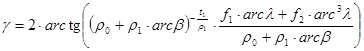
Representing the geographic quadrangle A), the minimal mean overall error  E_AK =0.00637  turns up when choosing  t₁=-0.995054, r₀=0.008385,  r₁=1.079275,  f₁=0.413701,  f₂=0.027033.

The radial function of the orthogonal pseudopolyconic projection

with pole as point:                                                                           r=r₁×arcb +r₂×arc²b ;

the distance  c  of the centre of the parallel  b  from the axis  x:      c=t₁×arcb+r

the angle  g  of the radius-vector pointing to the image of the point  (b,l)  enclosing with the central meridian:

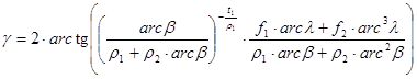
Representing the geographic quadrangle B), the minimal mean overall error  E_AK =0.00442

turns up when choosing  t₁=-0.994114, r₁=0.880601,  r₂=0.459705,  f₁=0.591129,  f₂=0.029848.

The parameter values giving the minimal mean overall errors  E_AK  were calculated by the "downhill simplex method" ([4]).

References

[1]       Bugayevskiy, L. M. – Snyder, J. P.: Map Projections. A Reference Manual. Taylor & Francis, London 1995.

[2]       Franċula, N.: Die vorteilhaftesten Abbildungen in der Atlaskartographie. Doktori disszertáció, Bonn 1971.

[3]       Haines, G. V.: The modified polyconic projection. In: Cartographica, 1981/1.

[4]       Press, W. H. - Teukolsky, S. A. - Vetterling, W. T. - Flannery, B. P.: Numerical Recipes. Cambridge Univ. Press 1986.

[5]       E@:@&\,&îñ;ïñ)ï:ñ;"H,<"H4R,F8"b 8"DH@(D"L4b. =,*D", ;@F8&" 1969.

[6]       Wagner, K.: Kartographische Netzentwürfe. Bibliographisches Institut, Mannheim 1962.

Figures

Figure 1:  The structure of the pseudopolyconic projection

Figure 2:  Canada on orthogonal pseudopolyconic projection with pole line.

Figure 3:  The European Union on orthogonal pseudopolyconic projection with pole as point.

Összefoglalás

Az Egyenlítőtől távol eső területek ábrázolására többnyire a parallelköröket körív formájában megjelenítő vetületeket (nevezetesen a valódi és képzetes kúpvetületeket) használják. Ekkor a fokhálózat merőlegessége gyakran előnyös a torzulások szempontjából. Ez a tulajdonság megvan a valódi kúpvetületeknél, valamint az ún. ortogonális polikónikus és pszeudopolikónikus vetületeknél.

Az ortogonális polikónikus vetületet korábban topográfiai térképeknél használták. Csak kevéssé alkalmas kiterjedt területek ábrázolásához, mert a torzulások a középmeridiántól távolodva gyorsan növekednek. Ha viszont a parallelkör képének r sugarát a polikónikus vetületekre jellemző tgb függvény helyett egy más függvénnyel (pl. egy polinommal) adjuk meg, akkor pszeudopolikónikus vetülethez jutunk. Legfeljebb másodfokú polinomot alkalmazva, a torzultság lényegesen csökkenthető.

Egy inkább K-Ny-i irányban kiterjedt A) területet és egy É-D-i irányban megnyúlt B) területet ábrázoltunk a de l'Isle-féle meridiánban hossztartó valódi kúpvetületben, ortogonális polikónikus valamint ortogonális pszeudopolikónikus vetületben. E vetületek paramétereit az  E_AK  Airy-Kavrajszkij-féle átlagos teljes torzultsági kritérium minimális értékéhez határoztuk meg a szimplex módszer segítségével. A pszeudopolikónikus vetületek  E_AK  értékei jelentősen kisebbek a többi vetületénél. A pszeudopolikónikus vetületeken belül a kétparaméteres sugárfüggvénnyel megadottak már elfogadhatóan pontos közelítést szolgáltatnak; a kritérium-érték nem csökken észrevehetően tovább három paraméteres sugárfüggvény esetén.

Az ortogonális pszeudopolikónikus vetület előnyös olyan földrajzi térképekhez, amelyek közepes vagy magasabb szélességen elhelyezkedő területeket ábrázolnak. A torzulások szempontjából hatékonyabban tudjuk alkalmazni, ha a terület kiterjedése É-D-i irányban nagyobb. Ebben az esetben a póluspontos változat  (r=r₁×arcb+r₂×arc²b)  kedvezőbb, főleg ha a pólus is ábrázolásra kerül. A pólusvonalas változat  (r=r₀+r₁×arcb)  akkor jobb, ha a pólustól távol eső vagy K-Ny-i irányban kiterjedtebb területet ábrázolunk.