Lecture notes Chapter 3

Transformations among the different types of coordinate systems on the spherical and ellipsoidal surfaces

During the practical use of coordinates coming from different types of coordinate systems, conversions are required among them.

Transformation between geographic and spatial rectangular (Cartesian) coordinates

The formulae below can be obtained from the definition of the geographic coordinates related to a right-handed Cartesian coordinate system, if the origins of the two coordinate systems concide, additionally the axis z and the polar axis coincide, too, moreover the unit at the axes is the same.

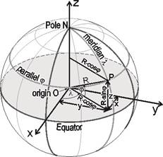
Sphere with radius R

                forward formulae:

reverse formulae:

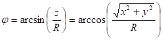
Ellipsoid with semi-axes  a  and  b

Formulae disregarding the elevation:

                forward formulae:

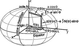
reverse formulae:

F can be expressed from the formula for Z  by rearranging it, in consideration of sinF:

                and

Formulae taking elevation  h  into consideration:

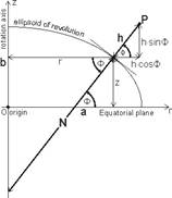
In the right triangle the length of the hypotenuse equals:

forward formulae:

reverse formulae (which are applied in the satellite navigation):

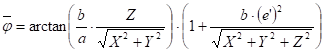
a) by iteration (Bowring) with the help of the reduced latitude j

initial values  and for reduced latitude j  and geographic latitude F:

                                     and

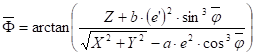
then the next three joint formulae:

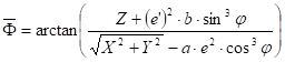
should be executed repeatedly one after the other, until the deviation between the last and the last but one latitude value is smaller than the required accuracy. After sufficient number of steps an approximative value of the geographic latitude F will be obtained.

The elevation h originates from the formula for Z:

,

and again

.

b) with accurate algorithm (Borkowski):

the distance of the point P from the ellipsoid’s rotation axis will be denoted by  ;

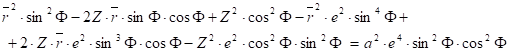
                               Let  h  be expressed both using both this formula and the above formula for  Z:

,   that is

The square root will be removed with the help of squaring. After it, the equation will be multiplied by the denominators:

Then this equation will be rearranged and divided by  cos⁴F meanwhile the identity

is applied. A quartic equation of  tanF will be got:

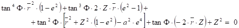
It can be solved exactly e.g. by the Ferrari’s method.

Finally the longitude L and the elevation h can be got similarly to the Bowring method above.

If the origins and/or the correspondent axes of the two coordinate systems do not coincide, and/or the unit of measurements at the axes differ, then coordinate transformation(s) can be required (translation, rotation, affine transformation in other words affinity, similarity in other words scaling up and down).

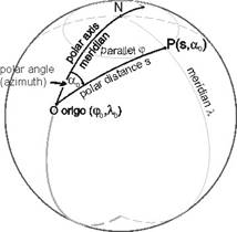
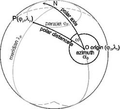
Superficial polar coordinate system on the spherical and ellipsoidal surfaces

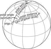
All the three types of regular surfaces taken for approaching the Earth’s surface – the plane, the sphere and the ellisoid – are surfaces of revolution, so the superficial polar coordinate system can be defined on them. As usual, the polar distance is provided by the geodesic line (the shortest surface line) connecting the origin O and the point P. In a plane, the geodesic lines are straight line segments, and on a spherical surface,  the geodesic lines are great circle arcs, while on an ellipsoidal surface the geodesic lines are in general more difficult curves.

The Clairaut’s theorem gives an important property of the points along a geodesic line on every surface of revolution, so in plane, on sphere and ellipsoid. Namely at every point P of latitude F, lying on the geodesic line, the product of the radius r(F) of the parallel crossing the point P and the sine of the azimuth  a  of the tangent to the geodesic line at the point  P, does not depends on the location of the point P. In formula:

along a geodesic line.

Conversely, if the product  r(F)×sina  is constant along a line, and if no part of the line is part of some parallel on the surface of revolution, then this line is a geodesic one.

Let a superficial polar coordinate system be defined on the surface of both the sphere and ellipsoid.

Sphere:

The polar axis coincides with a part of a meridian (great circle arc , geodesic line), starting from the appointed origin O. The polar distance comes from the length of the great circle arc connecting the origin O and the point P. The polar angle (azimut) can be measured at the origin O between the tangent lines of the meridian and the geodesic line, exeptionally clockwise. Problems connected to these coordinates lead up to spheric trigonometry calculations.

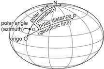
Ellipsoid:

The polar axis coincides with a part of a meridian (ellipse , geodesic line), starting from the origin O. The polar distance is the length of an arc of geodesic line on the surface of the ellipsoid connecting the origin O and the point P. The polar angle is the angle measured at the origin O between the tangents of the polar axis and the geodesic line, clockwise, too.

The principal problems of geodesy - transformation between geographic coordinates and superficial polar coordinates

First (direct) geodetic problem

Sphere

Given the polar distance (arc length s) of the point P from the origin O(j₀, l₀) and its azimuth a₀ on spherical surface, and asked the geographical coordinates j_P and l_P of P. Starting from the spherical triangle NOP  (where N is the pole), the cosine rule for sides can be applied:

(s/R  is the central angle (in radians) belongig tho the arc s in the great circle with radius R). Expressing the latitude j_P:

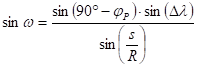
The longitude difference  Dl = l_P-l₀  results from the law of sines:

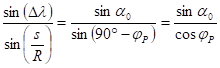
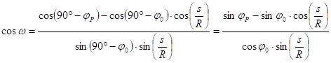
To calculate  Dl  correctly its cosine is required, too. It comes from an other cosine rule for sides:

and rearrangig this formula:

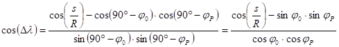
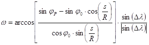
 So

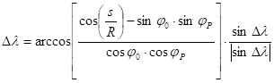
(If some factor in the denominator equals zero, Dl can be obtained without this formula.)

Finally

Ellipsoid

Given the polar distance (arc length s) of a geodesic line connecting the origin O(F₀, L₀) and the point P, in addition its azimuth a₀ on ellipsoidal surface;  asked the geographical coordinates  F_P  and  L_P  of  P. Consider these coordinates and the azimuth of the points as a function of  s:

F(s), L(s) and a(s)

The Legendre method is based on power series expansion of these functions at  s=0. It needs the derivatives of the functions, originating from the ellipsoidal triangle ABT created by an infinitely small arc AB of the geodesic line with the length of Ds, an arc of a parallel crossing B and an arc of a meridian crossing A. The meeting point of the parallel and the meridian will be denoted by T.

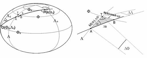
 The meridian arc AT belongs to the central angle DF, its length is about M(F)×DF. The small triangle ABT looks approximately the same as a planar one, so

On the other hand, the arc BT is part of a parallel of radius  N(F)×cosF, and it belongs to the central angle DL. With the help of its length we get:

The azimuth  a  should be considered as the function of  s, too. Here we will use Clairaut’s theorem, concerning surfaces of revolution. According to this, the product of radius of parallels  r  and the sine of the azimuth  a  is constant along the geodesic line on a surface of revolution, so:

Its derivative with respect to  s  is the following:

Substituting the formulae of  N(F),  M(F)  and  dF/ds  into the above equation and rearranging it:

These derivatives provide the first term of power series in  s=0,  F=F₀  and  a=a₀. If we continue the differentiation with respect to  s, the derivatives at the point O(F₀, a₀) give the coefficients of the power series.

In the geodesy at least five terms of these power series have to be calculated because of the slow convergence, so this method requires improvements.

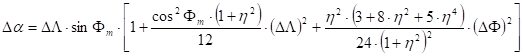
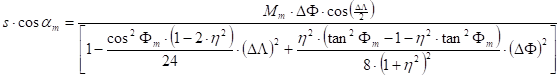
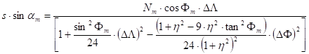
The Gauss’s mid-latitude method being based upon the previous one demands less calculations, because it expands the power series about the midpoint of the geodesic line  OP. We get the recursive formulae from a longer, here not detailed deduction:

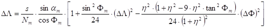
where DF and DL are the coordinate differences between the origin O and the actual approximation of the endpoint P:

              and        ,

F_m is the latitude and a_m is the azimuth calculated by averaging of the values refering to the origin and the actual approximation of the endpoint P:

,  , 

 furthermore   ,  ,  and  

(e’ is the second eccentricity of the ellipsoid: ).

This system of equations can be solved by iteration. We use on the right-hand of the equations e.g.  Dj  and  Dl  as initial values originating from the calculation with the osculating sphere belonging to F_m, instead of coordinate differences DF and DL. The expressions in brackets on the right-hand side became sufficiently accurate after one-two iterations, on this way only their multiplayer factor varies.

Second (inverse) geodetic problem

Sphere

Given the geographical coordinates j_P  and l_P  of the point P on spherical surface, and asked the polar distance (arc length s) of the point P from the origin O(j₀, l₀) and its azimuth a₀. From the cosine rule for sides:

where Dl=l_P-l₀

The arc length s can be expressed from this formula.

Let the interior angle w lying next to the point  O  of the spherical triangle  NOP be taken,  to calculate the azimuth  a₀. From the law of sines:

From the cosine rule of sides:

and rearranging this formula:

So

If point P is located to east from the meridian of the origin O, then

 ,

else

.

Ellipsoid

Given the geographical coordinates  F_P  and  L_P  of  P, and asked the polar distance (arc length  s)  of geodesic line which connects the origin  O(F₀, L₀)  and the point  P, and given its azimuth  a₀  on ellipsoidal surface. The usual solution of the inverse geodetic problem starts from the Legendre method applied earlier in the direct problem, too. Its improvement, the Gauss’s mid-latitude method provides here formulae which give the correct result without any iteration:

(We use the denotations again

,  , 

,  , 

then  ,  ,  and    ,  furthermore     and   .)

The azimuth  a_m  and the arc length  s  come from the formula

 ,

and

Finally, subtraction of  a_m  from  Da/2  provides the azimuth  a₀  at the initial point of the geodesic line, and, besides the addition of  a_m  and  Da/2  gives the azimuth  a_P  in its endpoint.

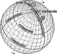
Metacoordinates, metagraticule on the sphere

The geographical coordinates on the sphere generate a graticule with the help of parallels and meridians. A new reference system, similar to the geographical coordinate system will be got by its rotations. It can be favourable for describing some map projections, and calculating map coordinates in this projections.

Let a point N* be selected on the surface of the sphere („metapole”). A spatial polarcoordinate system where the origin in the sphere’s center and a polar axis crossing N*,  defines „metalatitudes” by the polar angle, and a fixed semi-plane bounded by the polar axis defines „metalongitudes” for the point P. These „metacoordinates” establish a „metagraticule”, where the great circles of the sphere passing starting from N* are the „metameridians”, and the small circles of the sphere whose centre is on the metapolar axis are the „metaparallels”. (The metaparallel with metalatitude 0° - the „metaequator”  – is exceptionally a great circle, of course.) The prime metameridian mostly crosses one of the original poles for practical reason.

The ellipsoid of revolution has not rotational symmetry around any arbitrary axis differing from its own rotation axis, so a metacoordinate system and a metagraticule can not be defined on it.

Transformation between the geographical coordinates and the metacoordinates

A) Transformation by the help of coordinates (j₀,l₀) of the metapole N* and the prime metameridian

This task emerges mostly in that case, when the points with coordinates to be transformed are located in the surroundings of the metapole. Let the prime metameridian be directed now to the pole N.

a) Given the coordinates (j_P,l _P) of the P, and asked its metacoordinates (j*,l*)

This case brings us back to the inverse geodetic problem. The origin  O  corresponds to the metapole  N*, the spherical distance  s  (or rather the central angle  s/R) corresponds to the complementary angle of the metalatitude  j*, and the azimuth  a  corresponds to the metalongitude  l* but the angles azimuth and metalongitude are oppositely signed. So

(the longitude difference:  Dl=l_P-l₀).

and

If any factor in the denominator of this formula equals zero, then a simpler formula can be applied:

· In the case of N*ºN and N*ºS (j₀=±90°) the metalongitude differs in an additive constant angle and by chance in its sign from the longitude (l*=l+const  or  l*=–l+const).

· The metalongitude is indeterminate if the point P  and the metapole  N*  coincide (j*=±90°), so an arbitrary metalongitude  l* can be attributed to point P.

· It is easy to determine the metalongitude  l*, if the point P is located on the bimeridian crossing both  N  and  N*, that is  =0°,   |Dl|=180°  or |Dl|=360°. In this case  l*=0°  or l*=±180° is valid depending on the location of the point P on the bimeridian.

If none of these conditions is satisfied then the formula above works.

b) Given the metacoordinates  (j*,l*) of the point P, and asked its coordinates  (j,l)

This case is originated in the direct geodetic problem. The metapole  N*  corresponds to the origin  O the complementary angle of the metalatitude  j*  corresponds to the central angle  s/R, and the metalongitude  l*  corresponds to the negative of the azimuth  a₀  or to  360°–a₀. So, with substitution of  90°-j* into s/R  and  l* into –a₀,

                Similarly to the above suppositions, that

· j₀¹90° (else the metalongitude  can be obtained from the longitude by addition of a constant angle and possibly by a change in its sign);

· j_P¹±90° (else an arbitrary metalongitude  l* can be attributed to the point P);

· l*¹0°,   |l*|¹180°  and  |l*|¹360° (else  Dl=0°  or  Dl=±180°, depending on the position of the point P on the bimeridian crossing  N  and  N*):

the formula

                can be got, and finally  .

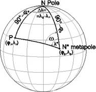
B) Transformation by the help of the intersection point K of the metaequator and the prime metameridian, completed with its direction

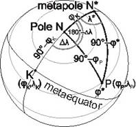
This task is generally applied when the points with coordinates to be transformed are located in the surroundings of the metaequator. Let the prime metameridian be crossing both the metaequator at the point K with coordinates  j_K and l_K and the pole N.

a) Given the coordinates (j_P,l_P) of the point P; asked its metacoordinates (j*,l*)

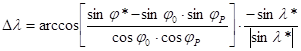
This case leads to a spherical trigonometric problem. Let the quarter-circular arc starting from K through N with the end point N* be considered. The PNN* spherical triangle with the sides one by one:  j_K,  90°-j* and  90°-j_P, with the angle 180°-Dl lying next to the vertex N, where  Dl=l_P-l₀  and the angle  l* (with sign) lying next to the vertex N*.  From the cosine rule for sides concerning side PN*; then we obtain

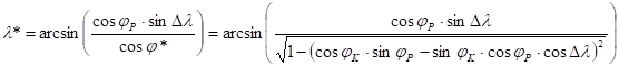
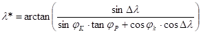
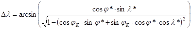
The next formula which can be obtained from tan(l*)  is in use more frequently. Applying the law of sines above for  sin(l*),  and the cosine rule concerning side  PN  for cos(l*):

Simplifying by cosj*, and dividing both the numerator and the denominator by cos(j_P):

b) Given the metacoordinates (j*,l*) of the point P, and asked its coordinates (j,l)

This case can be solved by spherical trigonometry, too. Take the PNN* spherical triangle again. It comes from the cosine rule for sides concerning the side opposite to the vertex N*:

Let us apply the law of sines refering to the vertices N and N*. Similarly to the above mentioned operations, we get:

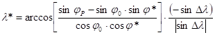
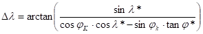
An other formula for  Dl  can be obtained from the  tan(Dl), too, writing now the cosine rule for sides concerning the side opposite to the vertex N. After expressing  cos(Dl)  from this, substituting the expression above to  sinj_P and using the formula of sin(Dl), the next relationship will be acquired:

Simplifying by cos(j_P), and dividing both the numerator and the denominator by cos(j*):

and finally