Conversions between map coordinates of different projections

The Earth sciences and the engineering use large data of map coordinates originating from measurements, coming from different ages. The location of these data occurs in diverse map coordinate systems, which causes difficulties by the integration of data. Therefore the conversion of particular map coordinates to another one is often required.

These conversions can be classified whether the geodesic datums and projections of the source and target coordinate systems are identical or diverse.

Conversions by the coordinate method

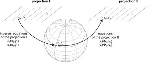
This method use the inverse projection equations for the calculation from the source map coordinates to the geographical coordinates, and the direct projection equations of an other projection for the calculation from the geographical coordinates to the map coordinates concerning the target projection.

• Identical datums, identical projections

This case covers the conversions between neighbouring Gauss-Krüger or UTM zones, neighbouring WAC sheets. The source projection and the target one have the same equations, only the longitudes of the midmeridian (or the true scale parallels in the case of Lambert conformal conical projection) differ in them.

The Gauss-Krüger maps contain the intersections of the map frame and the grid lines of the neighbouring zone, so the converted coordinates can be measured on the map with limited accuracy, and the calculations can be avoided.

• Identical datums, different projections

Such case comes into existence e.g. in conversion between Lambert conformal conical (WAC) coordinates and old UTM coordinates, as both projections are based upon the Hayford or lately the WGS84 ellipsoid. The ellipsoidal coordinates derive from the source map coordinates by the inverse projection equations, and then the target coordinates can be obtained by the target projection equations.

• Different datums, identical projections

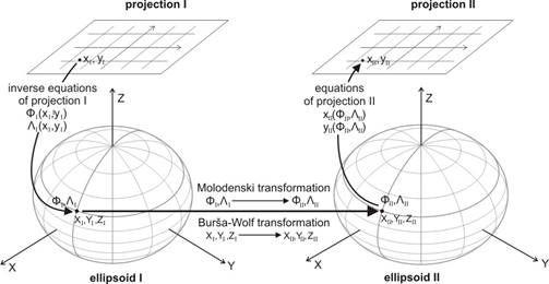
If two neigbouring countries use the same projection for their map system, but with different geodesic datum, then on the area near the frontier the inverse projection equations provide the ellipsoidal coordinates, which can be converted onto the other datums (e.g. either by the Molodenski or the Burša-Wolf transformation), finally the target projection equations give the target coordinates.

• Different datums, different projections

In most of the practical cases this general version is presented. After calculating the geographical coordinates on the ellipsoid from the source map coordinates, a conversion of these ellipsoidal coordinates onto the other ellipsoid follows with help of fitting points, finally the projection equations give the target map coordinates.

Conversion between map coordinates of different projections by polynomials

Regardless of the mathematical relationships between the source and target map coordinates and the correspondent geographical coordinates, it is possible to carry out simplified conversion between the map coordinates by poynomials.

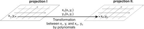
Denoted the source map coordinates by  x_I, y_I and the target ones by x_II, y_II, the connections between the correspondent coordinates are given as functions

which can be approximated by polynomials of the source map coordinates. The approximation needs fitting points with their correspondent map coordinates, and the error depends partly on the degree of the polynomials. The simplest case is the linear polynomial:

where A₀, A₁, A₂ and B₀, B₁, B₂ are constant coefficients, and their determination needs 3 fitting points. Substituting the correspondent coordinates in the equations above, 3 linear equations can be obtained for both the coefficients A_i and B_i (i=0,1,2):

   (i=1,2,3)

   (i=1,2,3)

The solution of these systems of equations provides the coefficients, and so the polynomials of the conversion. By the way, this conversion includes a translation by a vector of (A₀ , B₀) and approximately a rotation of the map plane. Using these formulae for the conversion of an arbitrary point  x_I, y_I , they will be accurate only in the fitting points, and the error increases in general diverging from them on the source map plane.

The accuracy of conversion can be improved by raising the degree of the polynomials. The quadratic approaching polynomials are the following:

Here 6 fitting points are required for the determination of the coefficients A_i and B_i (i=0,1,2,…,5). Substituting the correspondent coordinates into these equations, two linear systems of equations can be got for the coefficients:

       (i=1,2,…,6)

       (i=1,2,…,6)

Similarly to the linear case, the solution of these systems of equations provides the coefficients, and so the polynomials of the conversion. The result of the conversion of an arbitrary point  x_I, y_I given by this equations is accurate in the fitting points, but the error in other points can be smaller as in the linear case.

The degree of the approximating polynomials can be raised further, but the required number of the fitting points raises, too:

degree of the polynomials	1	2	3	4	5
required number of the fitting points	3	6	10	15	21

The further increase of the degree of the polynomials is not recommended because of the unpredictable behaviour of the approximated coordinates farther from the fitting points. If the number of the available fitting points is higher than the required, the coefficients can be determined by the method of least sum of squares. In this case the conversion results in smaller errors in the areas among the fitting points, but it is not quite accurate in the fitting points. (This calculation needs a solution of linear systems of equations, too.)