Map projections with favourable distortions

The map distortions

The surface of the Earth, or to be more precise a curved surface approximating the Earth, can be represented on map, which is – either a paper map or a screen map – a planar surface. Therefore the map making involves a mapping from the curved surface in question to the plain. For the easier mathematical handling, this curved plane has to be regular, continuous and describable by formulae, so it is commonly sphere or ellipsoid of revolution. It is parametrized by geographical coordinates  j and l, and the map plain mostly by (cartesian) rectangular coordinates x and y.

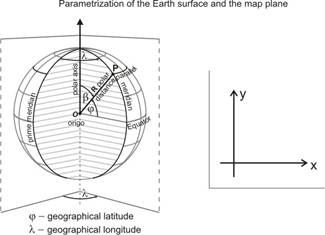
The calculation of mapping is usually carried out by the functions of two variables x(j,l) and y(j,l) (the so called „projection equations”). These functions are expected to be injective, two times continuously differentiable and describable by formulae or series.

Some measurable quantitative attributes of the Earth surface objects to be represented (e.g. arcs, surface figures, directions) change during the mapping, so these quantities are different on the map, which makes the quantitative map use difficult in practice. The most misleading are the changes of the lengthes, the areas and the angles. These changes are the so called map distortions, whose measure comes from the quotients of the quantites on the map and the the correspondent ones on the curved surface. The basic formulae concern to a point of the map (and they are actually limits):

scale distortion:  ,  where ds and ds’ are infinitesimally small arcs on the curved surface and on the map; it depends on the local direction of the arc;

area distortion:  ,  where f and f ’ are infinitesimally small pieces of the curved surface and of the map.

angular distortion:  ,  where d and d’ are angles on the curved surface and on the maps. (The angle of two intersecting arcs is defined by the angle of their tangent in the cross point).

It means, if a particular distortion does not come off in a point of the map, the value of this distortion equals 1. If the quantity in question is greater on the map, than on the curved surface, the value of this distortion is greater than 1, else it is smaller than 1.

Calculation of the distortions in a point of the map

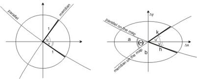
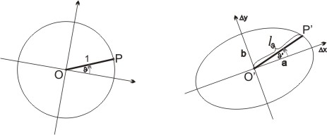
In most of the cases the calculation of the distortions is difficult on the basis of their definition. From practical point of view other formulae are more appropriate, which are based on the projection equations, or more precisely on their partial derivatives. The distortions here depend straight on the maximal and the minimal scale distortions (denoted by a and b), whose directions are perpendicular to another. As intermediate quantities the graticule distortions need to be used. These quantities and their relation with the graticule are demostrated by the Tissot’s indicatrix.

The graticule distortions are in case of sphere with radius R:

scale distortion h along the parallel of latitude j: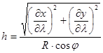           

scale distortion k along the meridian (of longitude l):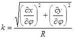  

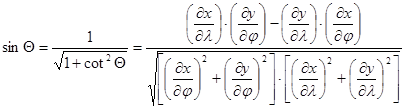
                the angle Q included by the meridian and the parallel in a point of the map:                                                    ,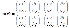

and 

The formulae for the maximal and minimal scale distortions a and b using the graticule distortions are the following:

and

The calculations of the maximal and minimal distortions a and b play an important role in the field of the map projections with optimal distortions.

Incidentally, the area distortion t  can be calculated directly by the graticule distortions, too:

The local direction of the maximal scale distortion includes angles u and v with the meridian and parallel arcs in a point of the sphere. They derive from the following formulae without their sign:

and

The formulae for the correspondent angles u’ and v’ in a point of the map:

            and       

while           and                   according to their definition.

The formulae of the distortions defined above are the following:

the area distortion t : 

the scale distortion l_J in a particular direction which includes an angle J with the direction of the maximal scale distortion a on the map:

the angular distortion i_J of a particular direction which includes an angle J with the direction of the maximal scale distortion a on the map:

the angular distortion i of an angle d between two arbitrary directions on the map (the angle d is composed as the difference of the angles m and n, the arm of which coincide with the direction of the maximal scale distortion a):

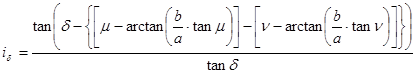
where  of the ;

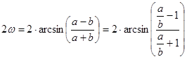
the distortion of an angle in a point of the map can be characterized also by the maximal change 2w of the angle in question:

Comparison of several projections in the light of the relevant distortion

After choosing the relevant distortion, which makes the map use confused, a method needs for the comparison and grading of map projections from the point of view of these distortion. Let’s consider some maps representing the same territory but prepared on different projections. After determining the measure of the distortion in the most possible and dispersed points of the map and evaluating these quantities, we want to get only one number assigned to the projection, and it characterizes the distortion of the map on the whole. The projections can be then ordered by these numbers.

Distortions and errors – characterizing the degree of the deformation in the points of a map

The map distortions can deviate from  1.0 (from the case of lack of distortions). The changes in the size of mapped objects are disadvantageous both in the case of increase and decrease. The degree of deviation from 1.0 – from the case of lack of distortions – is called error (and denoted by e²). Depending on the misleading distortion: scale error, area error and angular error can be examined.

· index numbers of local scale error (taking into consideration, that the scale distortion in a point of the map can depend on the direction which includes the angle J with the direction of the maximal scale distortion):

(Jordan)

(Jordan- Kavraisky)

· the index numbers of local area error:

     (Airy)

           (Kavraisky)

· the index numbers of local angular error:

            (Airy)

              (Kavraisky)

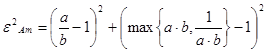
· the index number of the maximal angle change 2w, which is another sort of function of a/b, too:

· the value cot Q, which characterizing the change of the right angle included by the meridian and parallel in a point of the sphere surface, gives an other aspect of the angular error.

· the index numbers of the local complete error composed of the sum of angular and area errors:

   (Airy)

    (Airy modified)

          (Kavrayskiy)

· sometimes an other index is applied for this purpose:

         (Airy, James, Clarke)

(it is in fact the index number of the mean square deviation of the Tissot ellipse from its preimage);

· the index numbers of the local weighted complete error:

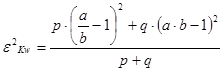    (Klingatsch)

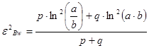        (Bayeva)

The evaluation of the local errors obtained from the whole territory of the map

The computed local errors must be taken into consideration altogether to get evaluative numbers, in order to obtain global error index number for comparing several map projections for reperesentation of the same territory. Two options are recommended:

Minimax principle – the aggregated error of the map is characterized by the maximum local error appearing on the map. The projection with the minimal maximum local error value will be regarded to be the best. The use of this principle is adequate, if we ignore the distortion of the map. It is suitable for large scale maps, because in this case the sizes measured on the map are transformed to real sizes merely by the map scale, and the distortions are omitted.

Principle of variations – the aggregated error of the map is characterized by the average of the local error values. The small scale maps represent in general a large part of the Earth, and the distortions are growing inevitably, therefore the application of the minimax principle is not suitable. Thus in the field of the geographic maps the projection with the minimal average error will be regarded to be the best. (The label „variation” originates from the mathematical solution of this task, which demands the use of calculus of variation.)

This course deals with the geographical maps of minimum error projections, so henceforward the principle of variations will be used for studying such projections.

Basic concepts in the study of minimum error map projections

For getting global error index numbers in the geocartography, a method is needed to average local errors on the territory to be represented.

Surface integral:

A domain (preferably a geographical quadrangle) T is appointed on a surface, and a number is assigned to the points of the domain, so a function is interpreted in the domain. After splitting the domain into small surface elements and multiplying the area of the elements by the value of the function at any points in this area, the limit of the sum of products is called the surface integral.

For example, a surface integral is defined by taking a part T of the surface and a local error index number e² assigned all to its points, which is denoted by

Using the definition above, the average E² of the local error index number e² referring to the territory T can be get from the formula

 (mean error index number, criterion of error)

where m(T) is the range of the domain T.

Knowing that Earth territories occuring in the practice can be approximated by sum of geographical quadrangles, it is enough to construct mean error index numbers only on this kind of parts of surfaces. In case of sphere we get the double integral:

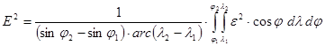
where the domain T is a geographical quadrangle  with the boundig parallels j₁ and j₂ and the bounding meridians l₁ and l₂ , and arcl denotes the angle l in radians.

When we compare the projections of two maps representing the same territory, then that projection is considered better, whose mean error index number E² is smaller. If we choose the projection with the smallest mean error from an infinite set of projections, we get the minimum error projection (with an other name projection of optimal distortion). The most favourable projection (that is the projection with the smallest mean error E²) chosen from the set containing all existing projections is called ideal projection. If we restrict the set to some subset of projections (e.g. equal-area projections, cylindrical projections, etc.), then when we choose from this subset we get the best cartographical projection.

The most important criteria of error are the following:

criteria of scale error:

           (Jordan)

          (Jordan-Kavrayskiy)

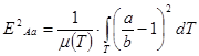
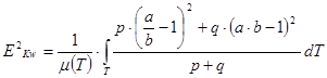
criteria of area error:

                        (Airy)

             (Kavrayskiy)

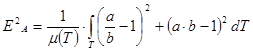
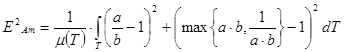
criteria of angular error:

              (Airy)

              (Kavrayskiy)

criteria of complete error:

       (Airy)

        (modified Airy)

       (Kavrayskiy)

sometimes an other criterion is applied here.

           (Airy, James, Clarke)

criteria of weighted complete error:

       (Klingatsch)

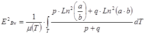         (Bayeva)

The enumerated criteria of error can be applied for the study of map projection errors with different efficiency. The choice from the criteria to be applied takes into consideration the claims made against the properties of the projection, the extent and situation of the territory to be represented, and possibly the distortion specialities of the projections which may come into question.

In case of distortional study of the whole Earth or a large territory, particularly the use of Kavraiskiy type error indices are proposed. The modified type Airy error indices give an appropriate result, too. The Airy-James-Clarke error index can be applied only in the neighborhood of the places without distortions. It is recommended to use Kavrayskiy type error indices if at least one of the a and b converges to the infinite.